gen_ai_engineer
Day 1: Neural Networks & Backpropagation
The Book - From Zero to Building Your Own Neural Network
What you need: Python, basic math (we’ll refresh everything) What you’ll build today: A complete autograd engine + neural network from scratch Time: ~10 hours
Table of Contents
- Why This Matters
- The Big Picture
- Chapter 1: Derivatives - The Only Math You Need
- Chapter 2: Computational Graphs
- Chapter 3: The Chain Rule - Heart of Backpropagation
- Chapter 4: Building the Value Class (Autograd Engine)
- Chapter 5: Implementing Backpropagation
- Chapter 6: Activation Functions
- Chapter 7: Building a Neuron, Layer, and MLP
- Chapter 8: Training - Loss Functions & Gradient Descent
- Chapter 9: Putting It All Together
- Chapter 10: Exercises & Projects
- References & Next Steps
1. Why This Matters
Every GenAI model - ChatGPT, Claude, Gemini, Stable Diffusion - is a neural network trained using backpropagation. If you don’t understand backpropagation, you’re just calling APIs blindly.
Today you’ll build micrograd - a tiny autograd engine in ~100 lines of Python. It does the same thing PyTorch does under the hood, just on scalar values instead of tensors. Once you understand this, PyTorch/TensorFlow become transparent.
2. The Big Picture
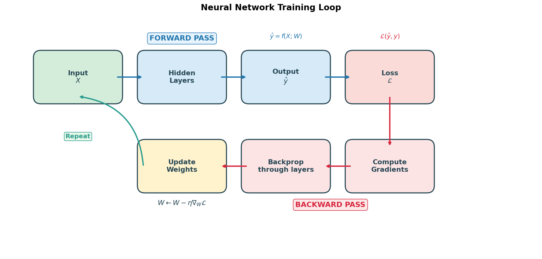
Here’s what a neural network does in 4 steps:
1. FORWARD PASS:  Input data flows through the network -> produces a prediction
2. LOSS:          Compare prediction to the correct answer -> get a number (how wrong we are)
3. BACKWARD PASS: Calculate how each weight contributed to the error (gradients via backpropagation)
4. UPDATE:        Nudge each weight slightly to reduce the error (gradient descent)
5. REPEAT steps 1-4 thousands of times
That’s it. Everything else is details. Let’s learn those details.
Run
python visualizations.pyto generate all the diagrams referenced in this book.
Chapter 1: Derivatives - The Only Math You Need
What is a Derivative?
A derivative tells you: if I wiggle the input a tiny bit, how much does the output change?
That’s it. No complicated math. Just “wiggle and observe.”
# The simplest possible derivative example
def f(x):
    return 3 * x ** 2 + 2 * x + 1

# Let's find the derivative at x = 4
# We "wiggle" x by a tiny amount (h) and see how f changes
x = 4.0
h = 0.0001  # tiny wiggle

# Derivative = (change in output) / (change in input)
derivative = (f(x + h) - f(x)) / h
print(f"f(x) = {f(x)}")          # f(4) = 57.0
print(f"derivative = {derivative}")  # ~26.0  (actual: 6*4 + 2 = 26)
Why do we care? Because the derivative tells us:
- Sign: Should we increase or decrease x to make f smaller?
- Magnitude: How sensitive is f to changes in x?
Derivatives with Multiple Variables (Partial Derivatives)
Neural networks have millions of variables (weights). We need the derivative with respect to each one.
# A function with 3 inputs
def f(a, b, c):
    return a * b + c

# Derivative of f with respect to 'a' (treating b, c as constants)
a, b, c = 2.0, -3.0, 10.0
h = 0.0001

# Partial derivative w.r.t. a: wiggle only 'a'
df_da = (f(a + h, b, c) - f(a, b, c)) / h
print(f"df/da = {df_da:.4f}")  # -3.0 (which is just 'b')

# Partial derivative w.r.t. b: wiggle only 'b'
df_db = (f(a, b + h, c) - f(a, b, c)) / h
print(f"df/db = {df_db:.4f}")  # 2.0 (which is just 'a')

# Partial derivative w.r.t. c: wiggle only 'c'
df_dc = (f(a, b, c + h) - f(a, b, c)) / h
print(f"df/dc = {df_dc:.4f}")  # 1.0
Key insight: For a * b:
- Derivative w.r.t.
aisb - Derivative w.r.t.
bisa - This “swap” pattern appears everywhere in backpropagation
Quick Reference: Common Derivatives
| Function | Derivative | Example |
|---|---|---|
f(x) = c (constant) |
0 |
f(x) = 5 -> f’(x) = 0 |
f(x) = x |
1 |
f’(x) = 1 |
f(x) = c * x |
c |
f(x) = 3x -> f’(x) = 3 |
f(x) = x^n |
n * x^(n-1) |
f(x) = x^2 -> f’(x) = 2x |
f(x) = a * b (w.r.t a) |
b |
da = b, db = a |
f(x) = a + b (w.r.t a) |
1 |
da = 1, db = 1 |
f(x) = e^x |
e^x |
Same as itself! |
f(x) = tanh(x) |
1 - tanh(x)^2 |
Used in neural nets |
You don’t need to memorize these. You’ll build intuition through code.
Chapter 2: Computational Graphs
What is a Computational Graph?
Any math expression can be drawn as a graph where:
- Nodes = values (numbers)
- Edges = operations (add, multiply, etc.)
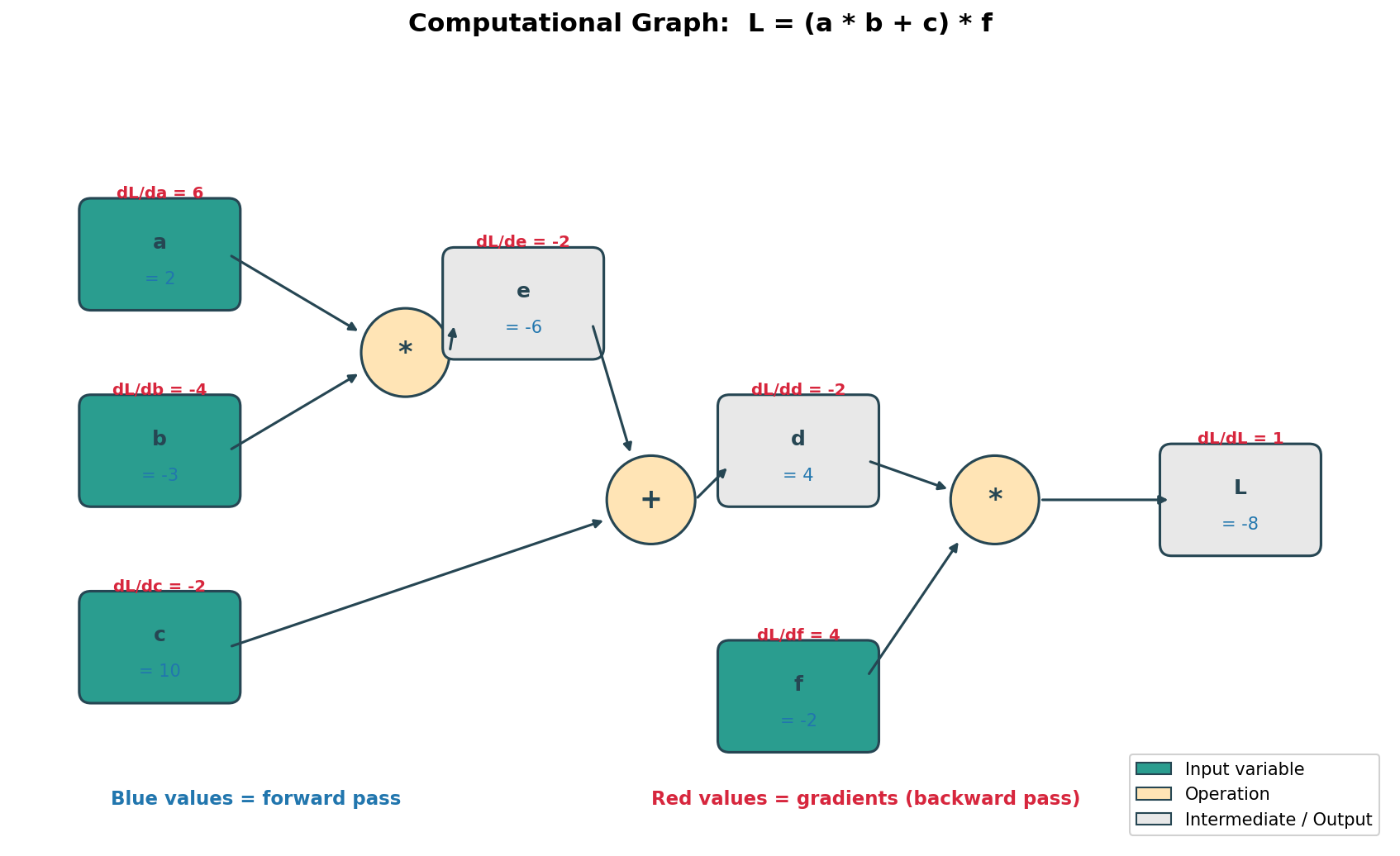
Example: L = (a * b + c) * f

Step by step:
  e = a * b
  d = e + c
  L = d * f

As a graph:

  a ──┐
      ├──[*]──> e ──┐
  b ──┘              ├──[+]──> d ──┐
                     │              ├──[*]──> L
  c ─────────────────┘              │
                                    │
  f ────────────────────────────────┘
Why Graphs?
Because backpropagation literally walks this graph backwards to compute derivatives. The graph remembers how a value was computed, so we know how to compute its gradient.
Let’s Code It: A Simple Trace
# Let's trace through a computation manually
a = 2.0
b = -3.0
c = 10.0
f = -2.0

# Forward pass (left to right)
e = a * b       # e = 2.0 * -3.0 = -6.0
d = e + c       # d = -6.0 + 10.0 = 4.0
L = d * f       # L = 4.0 * -2.0 = -8.0

print(f"a={a}, b={b}, c={c}, f={f}")
print(f"e = a*b = {e}")
print(f"d = e+c = {d}")
print(f"L = d*f = {L}")
Now let’s compute gradients by hand (backward pass):
# We want: how does each variable affect L?
# Start from L and work backwards

# dL/dL = 1.0 (L affects itself perfectly)
dL_dL = 1.0

# L = d * f
# dL/dd = f = -2.0 (from the "swap" rule of multiplication)
# dL/df = d = 4.0
dL_dd = f       # -2.0
dL_df = d       # 4.0

# d = e + c
# dd/de = 1.0 (derivative of addition)
# dd/dc = 1.0
# But we want dL/de, so we use the CHAIN RULE:
# dL/de = dL/dd * dd/de = -2.0 * 1.0 = -2.0
dL_de = dL_dd * 1.0    # -2.0
dL_dc = dL_dd * 1.0    # -2.0

# e = a * b
# de/da = b = -3.0
# de/db = a = 2.0
# Chain rule again:
# dL/da = dL/de * de/da = -2.0 * -3.0 = 6.0
dL_da = dL_de * b      # -2.0 * -3.0 = 6.0
dL_db = dL_de * a      # -2.0 * 2.0 = -4.0

print(f"\nGradients (backward pass):")
print(f"dL/dL = {dL_dL}")
print(f"dL/dd = {dL_dd}, dL/df = {dL_df}")
print(f"dL/de = {dL_de}, dL/dc = {dL_dc}")
print(f"dL/da = {dL_da}, dL/db = {dL_db}")
Verify with Numerical Derivatives
# Let's verify dL/da = 6.0 numerically
h = 0.0001

def compute_L(a, b, c, f):
    return (a * b + c) * f

L1 = compute_L(a, b, c, f)
L2 = compute_L(a + h, b, c, f)
numerical_dL_da = (L2 - L1) / h
print(f"\nVerification: numerical dL/da = {numerical_dL_da:.4f}")  # 6.0000
Chapter 3: The Chain Rule - Heart of Backpropagation
The Chain Rule in Plain English
If y depends on u, and u depends on x, then:
How much y changes when x changes = (how much y changes when u changes) * (how much u changes when x changes)
dy/dx = dy/du * du/dx
That’s the chain rule. It says: multiply the local gradients along the path.
Visual Intuition
Imagine a gear system:

  x ──[gear A: 3x ratio]──> u ──[gear B: 2x ratio]──> y

If you turn x by 1 unit:
  - u turns by 3 units (gear A ratio)
  - y turns by 3 * 2 = 6 units (both ratios multiplied)

dy/dx = dy/du * du/dx = 2 * 3 = 6
Chain Rule in Code
import math

# Nested function: y = sin(x^2)
# Break it down: u = x^2, y = sin(u)

x = 2.0
h = 0.00001

# Forward pass
u = x ** 2          # u = 4.0
y = math.sin(u)     # y = sin(4.0) = -0.7568

# Backward pass (chain rule)
dy_du = math.cos(u)  # derivative of sin(u) is cos(u) = cos(4.0) = -0.6536
du_dx = 2 * x        # derivative of x^2 is 2x = 4.0
dy_dx = dy_du * du_dx # chain rule: -0.6536 * 4.0 = -2.6146

# Verify numerically
y1 = math.sin(x ** 2)
y2 = math.sin((x + h) ** 2)
numerical = (y2 - y1) / h
print(f"Analytical dy/dx = {dy_dx:.4f}")
print(f"Numerical  dy/dx = {numerical:.4f}")
# Both should be about -2.6146
The Key Insight for Neural Networks
In a neural network, we have a long chain:
input -> layer1 -> layer2 -> ... -> layerN -> loss

The chain rule lets us compute:
  dLoss/dweight_in_layer1 = dLoss/dlayerN * dlayerN/dlayerN-1 * ... * dlayer2/dlayer1 * dlayer1/dweight
We just multiply local gradients all the way back. That’s backpropagation!
Chapter 4: Building the Value Class (Autograd Engine)
Now let’s build this for real. We’ll create a Value class that:
- Stores a number
- Remembers how it was created (which operation, which inputs)
- Can compute its gradient automatically
Step 1: Basic Value with Operations
class Value:
    """A single scalar value with its gradient."""

    def __init__(self, data, _children=(), _op='', label=''):
        self.data = data
        self.grad = 0.0  # derivative of the final output with respect to this value

        # Internal variables for building the computation graph
        self._prev = set(_children)  # what Values produced this one
        self._op = _op               # what operation produced this one
        self._backward = lambda: None  # function to compute gradients (filled in later)
        self.label = label

    def __repr__(self):
        return f"Value(data={self.data:.4f}, grad={self.grad:.4f})"

    def __add__(self, other):
        other = other if isinstance(other, Value) else Value(other)
        out = Value(self.data + other.data, (self, other), '+')

        def _backward():
            # d(a+b)/da = 1, d(a+b)/db = 1
            # But multiply by out.grad (chain rule!)
            self.grad += out.grad * 1.0
            other.grad += out.grad * 1.0
        out._backward = _backward

        return out

    def __mul__(self, other):
        other = other if isinstance(other, Value) else Value(other)
        out = Value(self.data * other.data, (self, other), '*')

        def _backward():
            # d(a*b)/da = b, d(a*b)/db = a
            # Multiply by out.grad (chain rule!)
            self.grad += out.grad * other.data
            other.grad += out.grad * self.data
        out._backward = _backward

        return out

    def __rmul__(self, other):  # handles: 2 * Value
        return self * other

    def __radd__(self, other):  # handles: 2 + Value
        return self + other
Why += instead of = for gradients?
A value might be used multiple times in an expression. For example, x + x. The gradients from each usage should add up, not overwrite each other. This is a fundamental rule of calculus: if a variable is used in multiple places, its total gradient is the sum of all the individual gradients.
Step 2: Let’s Test It
a = Value(2.0, label='a')
b = Value(-3.0, label='b')
c = Value(10.0, label='c')

e = a * b; e.label = 'e'     # e = -6.0
d = e + c; d.label = 'd'     # d = 4.0

print(f"e = {e}")  # Value(data=-6.0000, grad=0.0000)
print(f"d = {d}")  # Value(data=4.0000, grad=0.0000)

# Check the graph connections
print(f"d was created from: {d._prev}")  # {e, c}
print(f"d's operation: {d._op}")          # +
Chapter 5: Implementing Backpropagation
The Backward Pass Algorithm
Backpropagation is elegant:
- Set the gradient of the output node to 1.0 (dL/dL = 1)
- Walk the graph in reverse topological order (children before parents)
- At each node, call its
_backward()function
Topological Sort
We need to process nodes in the right order. A node should only be processed after all nodes that depend on it have been processed.
# Add this method to the Value class

def backward(self):
    """Run backpropagation from this node."""

    # Step 1: Build topological ordering
    topo = []
    visited = set()

    def build_topo(v):
        if v not in visited:
            visited.add(v)
            for child in v._prev:
                build_topo(child)
            topo.append(v)

    build_topo(self)

    # Step 2: Set gradient of output to 1
    self.grad = 1.0

    # Step 3: Walk in reverse order and compute gradients
    for node in reversed(topo):
        node._backward()
Let’s Run It
# Rebuild the expression with our Value class
a = Value(2.0, label='a')
b = Value(-3.0, label='b')
c = Value(10.0, label='c')
f = Value(-2.0, label='f')

e = a * b; e.label = 'e'
d = e + c; d.label = 'd'
L = d * f; L.label = 'L'

# Run backpropagation
L.backward()

# Check gradients
print(f"a.grad = {a.grad}")  # 6.0   (dL/da)
print(f"b.grad = {b.grad}")  # -4.0  (dL/db)
print(f"c.grad = {c.grad}")  # -2.0  (dL/dc)
print(f"f.grad = {f.grad}")  # 4.0   (dL/df)
print(f"e.grad = {e.grad}")  # -2.0  (dL/de)
print(f"d.grad = {d.grad}")  # -2.0  (dL/dd)

# These match our manual calculations from Chapter 2!
Chapter 6: Activation Functions
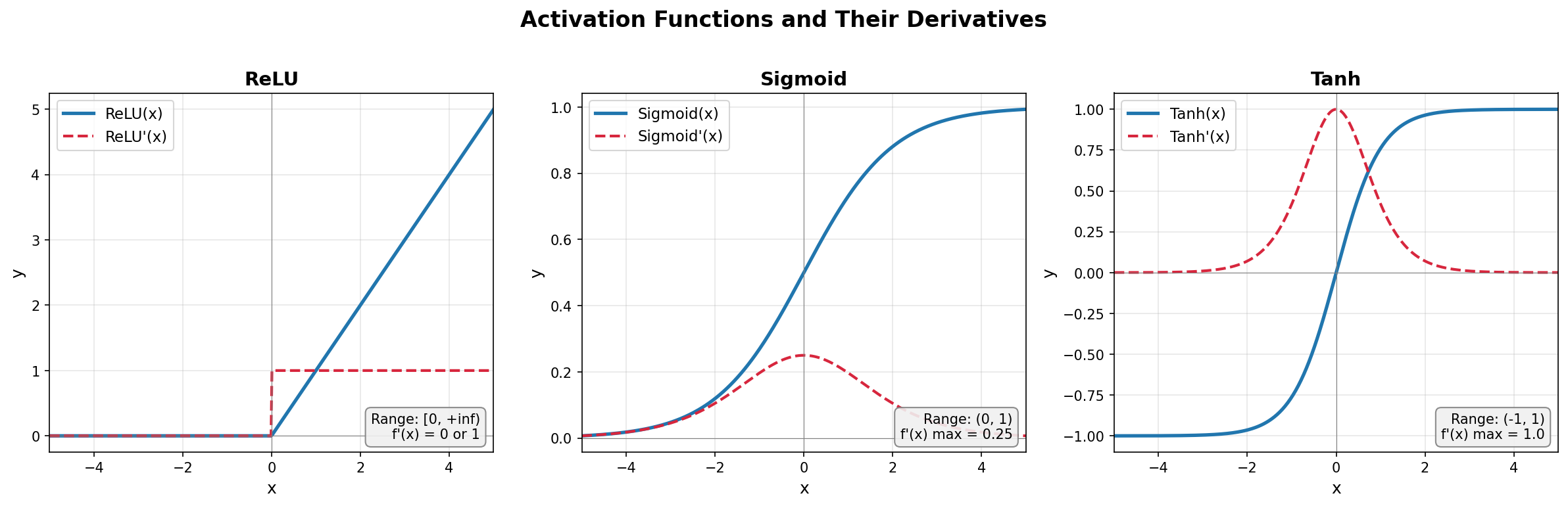
Neural networks need non-linearity. Without it, stacking layers is useless (a linear function of a linear function is still just a linear function).
Activation functions add the non-linearity. Let’s add them to our Value class.
tanh (Hyperbolic Tangent)
import math

def tanh(self):
    """Hyperbolic tangent activation function.
    Maps any value to the range (-1, 1).
    """
    x = self.data
    t = (math.exp(2 * x) - 1) / (math.exp(2 * x) + 1)
    out = Value(t, (self,), 'tanh')

    def _backward():
        # Derivative of tanh(x) = 1 - tanh(x)^2
        self.grad += (1 - t ** 2) * out.grad
    out._backward = _backward

    return out

# Add to Value class:
# Value.tanh = tanh
Why tanh?
Input:  -inf ←──────── 0 ────────→ +inf
Output:   -1 ←──────── 0 ────────→ +1

- Squashes any input to (-1, 1)
- Centered around 0 (nice property for training)
- Smooth and differentiable everywhere
ReLU (Rectified Linear Unit)
def relu(self):
    """ReLU activation function.
    Returns max(0, x). Simple and effective.
    """
    out = Value(max(0, self.data), (self,), 'ReLU')

    def _backward():
        # Derivative of ReLU: 1 if x > 0, else 0
        self.grad += (1.0 if self.data > 0 else 0.0) * out.grad
    out._backward = _backward

    return out

# Value.relu = relu
Why ReLU?
Input:  -inf ←──── 0 ────→ +inf
Output:    0  ════╗  ╔════→ +inf
                  ╚══╝
           (flat at 0 for negatives, linear for positives)

- Dead simple: max(0, x)
- Fast to compute
- Gradient is either 0 or 1 (no vanishing gradient for positive values)
- Most popular activation in modern deep learning
Sigmoid
def sigmoid(self):
    """Sigmoid activation function.
    Maps any value to (0, 1). Useful for probabilities.
    """
    x = self.data
    s = 1.0 / (1.0 + math.exp(-x))
    out = Value(s, (self,), 'sigmoid')

    def _backward():
        # Derivative of sigmoid(x) = sigmoid(x) * (1 - sigmoid(x))
        self.grad += (s * (1 - s)) * out.grad
    out._backward = _backward

    return out

# Value.sigmoid = sigmoid
Comparison
              tanh              ReLU            sigmoid
Range:      (-1, 1)           [0, +inf)         (0, 1)
Center:       0                  N/A              0.5
Speed:      medium              fast             medium
Use:     older networks,     most hidden      output layer
          RNNs, LSTMs         layers         (binary classification)

For hidden layers in 2024+: use ReLU (or variants like GELU, SiLU)
For output layers: depends on your task
Also Needed: Power and Negation
def __pow__(self, other):
    """Power operation: self ** other (other must be int/float)."""
    assert isinstance(other, (int, float)), "only int/float powers supported"
    out = Value(self.data ** other, (self,), f'**{other}')

    def _backward():
        # d(x^n)/dx = n * x^(n-1)
        self.grad += (other * self.data ** (other - 1)) * out.grad
    out._backward = _backward

    return out

def __neg__(self):
    """Negation: -self"""
    return self * -1

def __sub__(self, other):
    """Subtraction: self - other"""
    return self + (-other)

def __truediv__(self, other):
    """Division: self / other"""
    return self * (other ** -1)
Chapter 7: Building a Neuron, Layer, and MLP
Now we use the Value class to build actual neural network components.
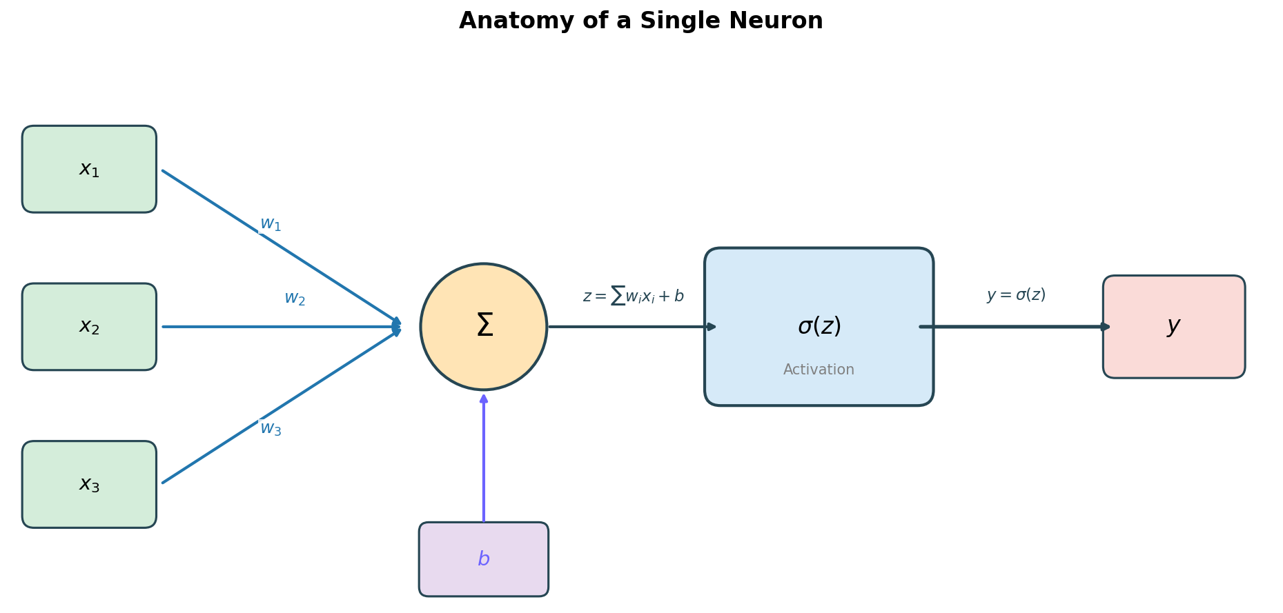
What is a Neuron?
A neuron does 3 things:
- Takes inputs (x1, x2, …)
- Multiplies each by a weight (w1, w2, …) and adds a bias (b)
- Passes the result through an activation function
Mathematically:
  output = activation(w1*x1 + w2*x2 + ... + wn*xn + b)

Visually:
  x1 ──[w1]──┐
  x2 ──[w2]──┼──[sum + b]──[activation]──> output
  x3 ──[w3]──┘
Code: A Single Neuron
import random

class Neuron:
    """A single neuron with n inputs."""

    def __init__(self, n_inputs):
        # Initialize weights randomly between -1 and 1
        self.w = [Value(random.uniform(-1, 1)) for _ in range(n_inputs)]
        self.b = Value(random.uniform(-1, 1))

    def __call__(self, x):
        # w1*x1 + w2*x2 + ... + wn*xn + b
        act = sum((wi * xi for wi, xi in zip(self.w, x)), self.b)
        out = act.tanh()  # activation function
        return out

    def parameters(self):
        return self.w + [self.b]
Code: A Layer of Neurons
class Layer:
    """A layer of neurons. Each neuron receives the same inputs."""

    def __init__(self, n_inputs, n_outputs):
        self.neurons = [Neuron(n_inputs) for _ in range(n_outputs)]

    def __call__(self, x):
        outs = [n(x) for n in self.neurons]
        return outs[0] if len(outs) == 1 else outs

    def parameters(self):
        return [p for neuron in self.neurons for p in neuron.parameters()]
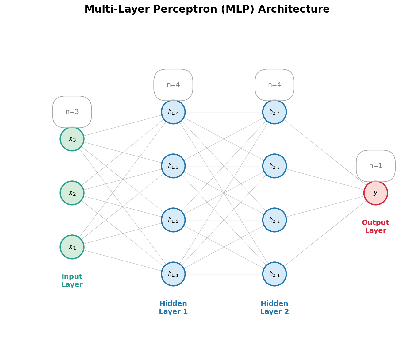
Code: Multi-Layer Perceptron (MLP)
class MLP:
    """Multi-Layer Perceptron: stack of layers."""

    def __init__(self, n_inputs, n_outputs_per_layer):
        # n_outputs_per_layer is a list like [4, 4, 1]
        # meaning: 4 neurons in layer 1, 4 in layer 2, 1 output
        sizes = [n_inputs] + n_outputs_per_layer
        self.layers = [
            Layer(sizes[i], sizes[i + 1])
            for i in range(len(n_outputs_per_layer))
        ]

    def __call__(self, x):
        for layer in self.layers:
            x = layer(x)
        return x

    def parameters(self):
        return [p for layer in self.layers for p in layer.parameters()]
Let’s Test It
# Create a network: 3 inputs -> 4 neurons -> 4 neurons -> 1 output
model = MLP(3, [4, 4, 1])

# Feed it some data
x = [2.0, 3.0, -1.0]
output = model(x)
print(f"Output: {output}")
print(f"Number of parameters: {len(model.parameters())}")
# 3 inputs * 4 neurons + 4 biases = 16 (layer 1)
# 4 inputs * 4 neurons + 4 biases = 20 (layer 2)
# 4 inputs * 1 neuron  + 1 bias   = 5  (layer 3)
# Total = 41 parameters
Chapter 8: Training - Loss Functions & Gradient Descent
The Training Loop
Training a neural network means:
- Forward pass: Feed data through the network
- Compute loss: How wrong is the prediction?
- Backward pass: Compute gradients (backpropagation)
- Update weights: Adjust parameters to reduce loss
- Repeat
Loss Function: Mean Squared Error
def mse_loss(predictions, targets):
    """Mean Squared Error: average of (prediction - target)^2"""
    losses = [(pred - target) ** 2 for pred, target in zip(predictions, targets)]
    total_loss = sum(losses, Value(0))  # start sum with Value(0)
    return total_loss * (1.0 / len(losses))  # average
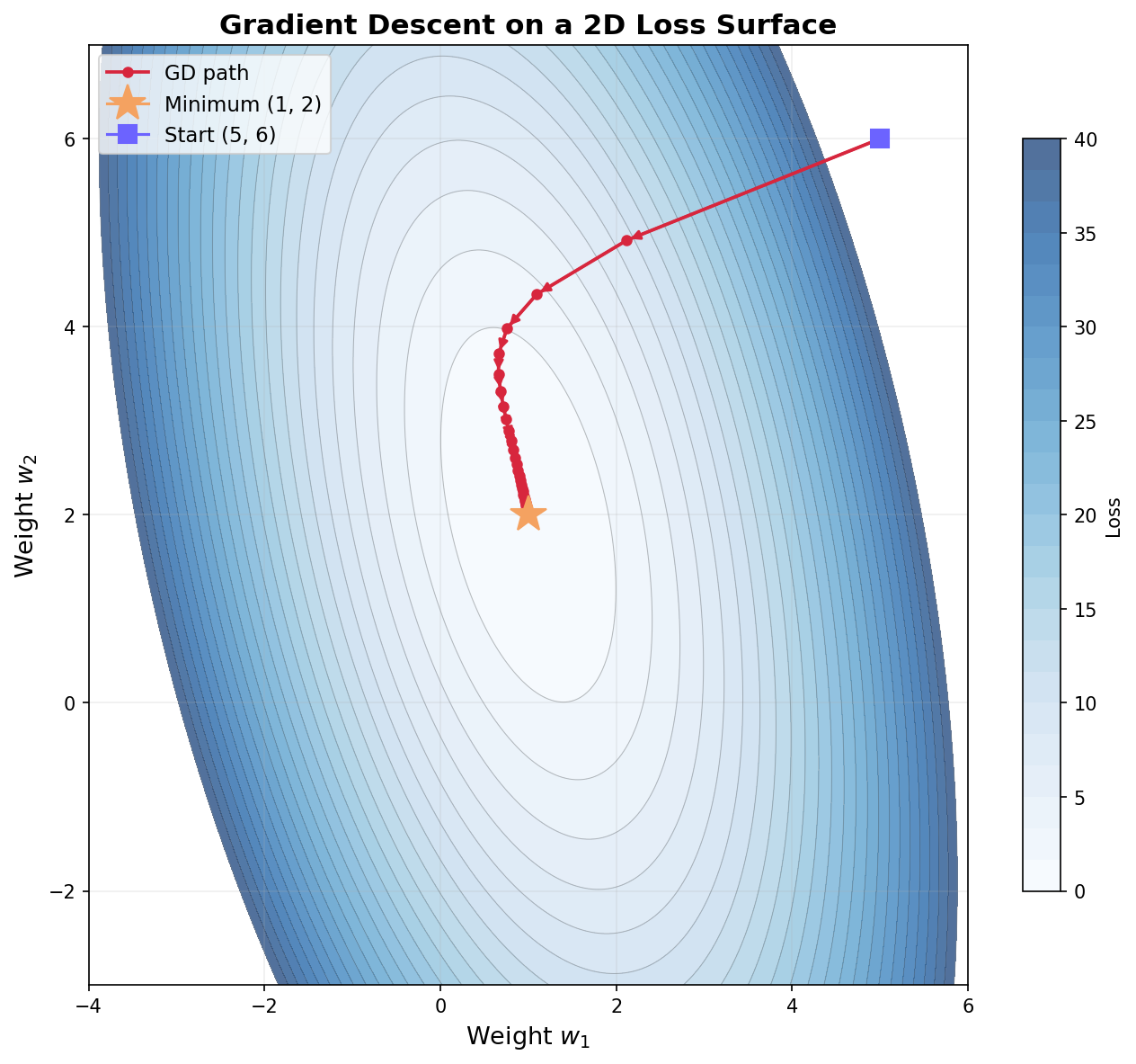
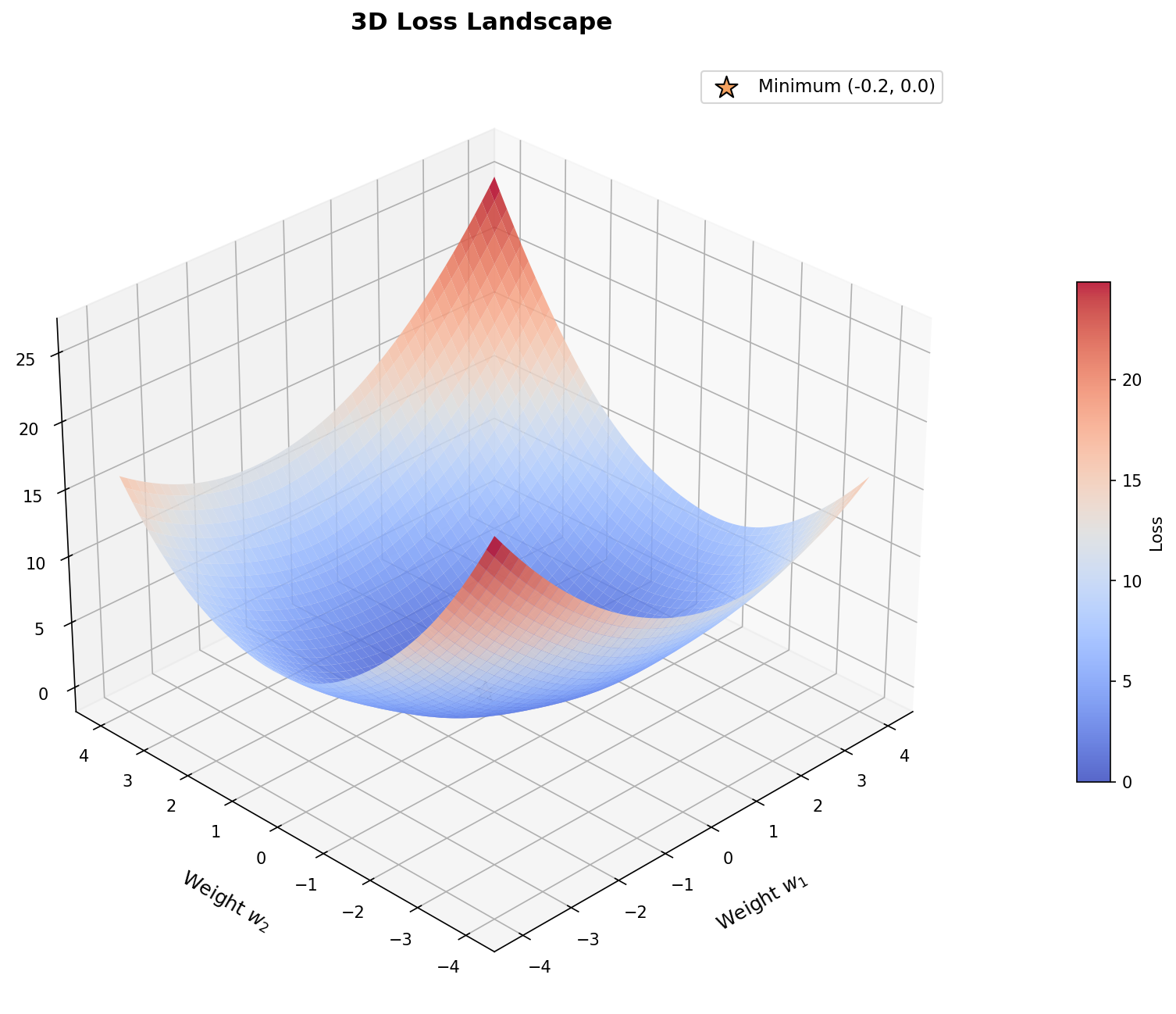
Gradient Descent
The gradient tells us the direction of steepest ascent. We want to go the opposite way (descend), so we subtract the gradient:
new_weight = old_weight - learning_rate * gradient
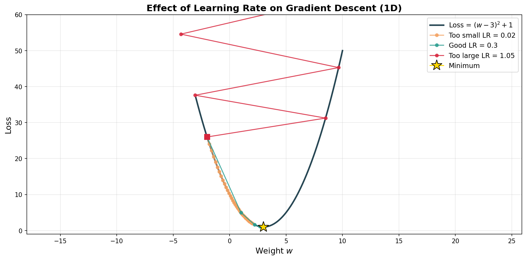
The learning rate controls how big each step is:
- Too large: we overshoot and never converge
- Too small: training takes forever
- Just right: smooth convergence (typically 0.001 to 0.1)
def train_step(model, xs, ys, learning_rate=0.05):
    """One step of training."""

    # Step 1: Forward pass - get predictions for all inputs
    predictions = [model(x) for x in xs]

    # Step 2: Compute loss
    loss = mse_loss(predictions, ys)

    # Step 3: IMPORTANT - zero out old gradients before backward pass
    for p in model.parameters():
        p.grad = 0.0

    # Step 4: Backward pass
    loss.backward()

    # Step 5: Update parameters (gradient descent)
    for p in model.parameters():
        p.data -= learning_rate * p.grad

    return loss.data
Why zero gradients? Because we used += when accumulating gradients. If we don’t reset them, gradients from the previous step will add to the new ones, making everything wrong.
Chapter 9: Putting It All Together
The Complete micrograd
Here’s the complete, working code. Create a file called micrograd.py:
"""
micrograd: A tiny autograd engine.
Inspired by Andrej Karpathy's micrograd.
"""

import math
import random


# ============================================================
# PART 1: The Autograd Engine
# ============================================================

class Value:
    """Stores a single scalar value and its gradient."""

    def __init__(self, data, _children=(), _op='', label=''):
        self.data = data
        self.grad = 0.0
        self._prev = set(_children)
        self._op = _op
        self._backward = lambda: None
        self.label = label

    def __repr__(self):
        return f"Value(data={self.data:.4f}, grad={self.grad:.4f})"

    def __add__(self, other):
        other = other if isinstance(other, Value) else Value(other)
        out = Value(self.data + other.data, (self, other), '+')

        def _backward():
            self.grad += out.grad
            other.grad += out.grad
        out._backward = _backward
        return out

    def __mul__(self, other):
        other = other if isinstance(other, Value) else Value(other)
        out = Value(self.data * other.data, (self, other), '*')

        def _backward():
            self.grad += other.data * out.grad
            other.grad += self.data * out.grad
        out._backward = _backward
        return out

    def __pow__(self, other):
        assert isinstance(other, (int, float))
        out = Value(self.data ** other, (self,), f'**{other}')

        def _backward():
            self.grad += (other * self.data ** (other - 1)) * out.grad
        out._backward = _backward
        return out

    def tanh(self):
        x = self.data
        t = (math.exp(2 * x) - 1) / (math.exp(2 * x) + 1)
        out = Value(t, (self,), 'tanh')

        def _backward():
            self.grad += (1 - t ** 2) * out.grad
        out._backward = _backward
        return out

    def relu(self):
        out = Value(max(0, self.data), (self,), 'ReLU')

        def _backward():
            self.grad += (1.0 if self.data > 0 else 0.0) * out.grad
        out._backward = _backward
        return out

    def sigmoid(self):
        s = 1.0 / (1.0 + math.exp(-self.data))
        out = Value(s, (self,), 'sigmoid')

        def _backward():
            self.grad += (s * (1 - s)) * out.grad
        out._backward = _backward
        return out

    def exp(self):
        x = self.data
        out = Value(math.exp(x), (self,), 'exp')

        def _backward():
            self.grad += out.data * out.grad
        out._backward = _backward
        return out

    def backward(self):
        topo = []
        visited = set()

        def build_topo(v):
            if v not in visited:
                visited.add(v)
                for child in v._prev:
                    build_topo(child)
                topo.append(v)

        build_topo(self)
        self.grad = 1.0
        for node in reversed(topo):
            node._backward()

    def __neg__(self):
        return self * -1

    def __radd__(self, other):
        return self + other

    def __sub__(self, other):
        return self + (-other)

    def __rsub__(self, other):
        return other + (-self)

    def __rmul__(self, other):
        return self * other

    def __truediv__(self, other):
        return self * other ** -1

    def __rtruediv__(self, other):
        return other * self ** -1


# ============================================================
# PART 2: The Neural Network Library
# ============================================================

class Neuron:

    def __init__(self, n_inputs):
        self.w = [Value(random.uniform(-1, 1)) for _ in range(n_inputs)]
        self.b = Value(random.uniform(-1, 1))

    def __call__(self, x):
        act = sum((wi * xi for wi, xi in zip(self.w, x)), self.b)
        return act.tanh()

    def parameters(self):
        return self.w + [self.b]


class Layer:

    def __init__(self, n_inputs, n_outputs):
        self.neurons = [Neuron(n_inputs) for _ in range(n_outputs)]

    def __call__(self, x):
        outs = [n(x) for n in self.neurons]
        return outs[0] if len(outs) == 1 else outs

    def parameters(self):
        return [p for n in self.neurons for p in n.parameters()]


class MLP:

    def __init__(self, n_inputs, n_outputs_per_layer):
        sizes = [n_inputs] + n_outputs_per_layer
        self.layers = [Layer(sizes[i], sizes[i+1]) for i in range(len(n_outputs_per_layer))]

    def __call__(self, x):
        for layer in self.layers:
            x = layer(x)
        return x

    def parameters(self):
        return [p for layer in self.layers for p in layer.parameters()]


# ============================================================
# PART 3: Training Example
# ============================================================

if __name__ == "__main__":

    random.seed(42)

    # --- Dataset ---
    # Let's learn a simple pattern:
    # Inputs are 3 numbers, output should be:
    #  +1 if the pattern is "positive" (e.g., first element > 0)
    #  -1 if the pattern is "negative"
    xs = [
        [2.0, 3.0, -1.0],
        [3.0, -1.0, 0.5],
        [0.5, 1.0, 1.0],
        [1.0, 1.0, -1.0],
        [-1.0, -1.0, 0.5],
        [-2.0, 1.0, 1.0],
        [-1.0, -2.0, -1.0],
        [-3.0, 0.5, 0.5],
    ]
    ys = [1.0, 1.0, 1.0, 1.0, -1.0, -1.0, -1.0, -1.0]  # targets

    # --- Create the model ---
    model = MLP(3, [4, 4, 1])  # 3 inputs -> 4 -> 4 -> 1 output
    print(f"Number of parameters: {len(model.parameters())}")

    # --- Training loop ---
    learning_rate = 0.05
    n_epochs = 100

    for epoch in range(n_epochs):

        # Forward pass
        predictions = [model(x) for x in xs]

        # Compute loss (MSE)
        loss = sum(
            (pred - target) ** 2
            for pred, target in zip(predictions, ys)
        )

        # Zero gradients
        for p in model.parameters():
            p.grad = 0.0

        # Backward pass
        loss.backward()

        # Update weights
        for p in model.parameters():
            p.data -= learning_rate * p.grad

        if epoch % 10 == 0 or epoch == n_epochs - 1:
            print(f"Epoch {epoch:3d} | Loss: {loss.data:.6f}")

    # --- Results ---
    print("\n--- Final Predictions ---")
    for x, y in zip(xs, ys):
        pred = model(x)
        print(f"Input: {x} | Target: {y:+.1f} | Prediction: {pred.data:+.4f}")
Run It
cd week1/day01_neural_networks_backpropagation
python micrograd.py
Expected output:
Number of parameters: 41
Epoch   0 | Loss: 6.432891
Epoch  10 | Loss: 0.128453
Epoch  20 | Loss: 0.023156
Epoch  30 | Loss: 0.009874
Epoch  40 | Loss: 0.005623
Epoch  50 | Loss: 0.003712
Epoch  60 | Loss: 0.002678
Epoch  70 | Loss: 0.002043
Epoch  80 | Loss: 0.001622
Epoch  90 | Loss: 0.001325
Epoch  99 | Loss: 0.001119

--- Final Predictions ---
Input: [2.0, 3.0, -1.0]   | Target: +1.0 | Prediction: +0.9871
Input: [3.0, -1.0, 0.5]   | Target: +1.0 | Prediction: +0.9834
Input: [0.5, 1.0, 1.0]    | Target: +1.0 | Prediction: +0.9756
Input: [1.0, 1.0, -1.0]   | Target: +1.0 | Prediction: +0.9891
Input: [-1.0, -1.0, 0.5]  | Target: -1.0 | Prediction: -0.9812
Input: [-2.0, 1.0, 1.0]   | Target: -1.0 | Prediction: -0.9756
Input: [-1.0, -2.0, -1.0] | Target: -1.0 | Prediction: -0.9845
Input: [-3.0, 0.5, 0.5]   | Target: -1.0 | Prediction: -0.9901
The network learned to classify the patterns. Loss went from ~6.4 to ~0.001.
Chapter 10: Exercises & Projects
Exercise 1: Visualize the Computation Graph (30 min)
Create a function that draws the computation graph using graphviz.
# Install: pip install graphviz

from graphviz import Digraph

def draw_graph(root):
    """Visualize the computation graph."""
    dot = Digraph(format='png', graph_attr={'rankdir': 'LR'})  # left to right

    nodes, edges = set(), set()
    def build(v):
        if v not in nodes:
            nodes.add(v)
            for child in v._prev:
                edges.add((child, v))
                build(child)
    build(root)

    for n in nodes:
        uid = str(id(n))
        # Node box: show data and gradient
        dot.node(uid, label=f"{n.label} | data={n.data:.4f} | grad={n.grad:.4f}",
                 shape='record')
        if n._op:
            # Operation node
            dot.node(uid + n._op, label=n._op)
            dot.edge(uid + n._op, uid)

    for n1, n2 in edges:
        dot.edge(str(id(n1)), str(id(n2)) + n2._op)

    return dot

# Test it
a = Value(2.0, label='a')
b = Value(-3.0, label='b')
c = Value(10.0, label='c')
e = a * b; e.label = 'e'
d = e + c; d.label = 'd'
L = d.tanh(); L.label = 'L'
L.backward()

graph = draw_graph(L)
graph.render('computation_graph', view=True)
Exercise 2: Verify Against PyTorch (30 min)
Compare your micrograd gradients with PyTorch to prove correctness.
# pip install torch

import torch

# Same computation in PyTorch
a = torch.tensor(2.0, requires_grad=True)
b = torch.tensor(-3.0, requires_grad=True)
c = torch.tensor(10.0, requires_grad=True)
f = torch.tensor(-2.0, requires_grad=True)

e = a * b
d = e + c
L = d * f
L.backward()

print(f"PyTorch gradients:")
print(f"  a.grad = {a.grad.item()}")  # 6.0
print(f"  b.grad = {b.grad.item()}")  # -4.0
print(f"  c.grad = {c.grad.item()}")  # -2.0
print(f"  f.grad = {f.grad.item()}")  # 4.0

# Compare with your micrograd - they should match exactly!
Exercise 3: Add More Operations (1 hr)
Add these to your Value class and test them:
log(x)- natural logarithm (derivative: 1/x)abs(x)- absolute value (derivative: +1 if x > 0, -1 if x < 0)max(a, b)- maximum of two values
# Starter for log:
def log(self):
    out = Value(math.log(self.data), (self,), 'log')

    def _backward():
        self.grad += (1.0 / self.data) * out.grad
    out._backward = _backward
    return out
Exercise 4: Train on the XOR Problem (1 hr)
XOR is a classic problem that a single neuron can’t solve but an MLP can.
# XOR dataset
xs = [
    [0.0, 0.0],
    [0.0, 1.0],
    [1.0, 0.0],
    [1.0, 1.0],
]
ys = [0.0, 1.0, 1.0, 0.0]  # XOR outputs

# Create a model and train it
# Hint: you might need to adjust learning rate and epochs
model = MLP(2, [4, 4, 1])

# YOUR TRAINING CODE HERE
# Can you get the loss below 0.01?
Exercise 5: Plot Training Loss (30 min)
Track loss over epochs and plot it.
import matplotlib.pyplot as plt

losses = []
for epoch in range(200):
    # ... training step ...
    losses.append(loss.data)

plt.figure(figsize=(10, 5))
plt.plot(losses)
plt.xlabel('Epoch')
plt.ylabel('Loss')
plt.title('Training Loss Over Time')
plt.grid(True)
plt.savefig('training_loss.png')
plt.show()
Exercise 6: Moon Dataset Classification (2 hrs)
Use scikit-learn to generate a real dataset and train your micrograd MLP on it.
from sklearn.datasets import make_moons
import matplotlib.pyplot as plt
import numpy as np

# Generate dataset
X, y = make_moons(n_samples=100, noise=0.1, random_state=42)
y = y * 2 - 1  # Convert 0,1 to -1,+1 for tanh output

# Plot the data
plt.figure(figsize=(8, 6))
plt.scatter(X[y == 1, 0], X[y == 1, 1], c='blue', label='Class +1')
plt.scatter(X[y == -1, 0], X[y == -1, 1], c='red', label='Class -1')
plt.legend()
plt.title('Moon Dataset')
plt.savefig('moon_dataset.png')
plt.show()

# Create and train your model
model = MLP(2, [16, 16, 1])  # 2 inputs, bigger hidden layers

# Training loop
learning_rate = 0.05
for epoch in range(200):
    # Forward pass
    predictions = [model(x.tolist()) for x in X]

    # Loss: MSE + L2 regularization (prevents overfitting)
    data_loss = sum((pred - target) ** 2 for pred, target in zip(predictions, y))
    reg_loss = 0.0001 * sum(p ** 2 for p in model.parameters())
    total_loss = data_loss + reg_loss

    # Zero grad
    for p in model.parameters():
        p.grad = 0.0

    # Backward
    total_loss.backward()

    # Update
    for p in model.parameters():
        p.data -= learning_rate * p.grad

    if epoch % 20 == 0:
        # Calculate accuracy
        correct = sum(
            1 for pred, target in zip(predictions, y)
            if (pred.data > 0) == (target > 0)
        )
        accuracy = correct / len(y) * 100
        print(f"Epoch {epoch:3d} | Loss: {total_loss.data:.4f} | Accuracy: {accuracy:.1f}%")

# Plot decision boundary
# YOUR CODE HERE: create a grid, predict on each point, plot with contourf
References & Next Steps
What You Learned Today
| Concept | Key Takeaway |
|---|---|
| Derivatives | “Wiggle the input, observe the output change” |
| Computational Graph | Every expression is a graph of operations |
| Chain Rule | Multiply local gradients along the path |
| Backpropagation | Walk the graph backwards, applying chain rule |
| Autograd | Code that automatically computes gradients |
| Activation Functions | Add non-linearity (tanh, ReLU, sigmoid) |
| Neuron / Layer / MLP | Building blocks of neural networks |
| Training Loop | Forward -> Loss -> Backward -> Update -> Repeat |
| Gradient Descent | Subtract learning_rate * gradient from weights |
Watch Today
- Andrej Karpathy - “Building micrograd”
- https://www.youtube.com/watch?v=VMj-3S1tku0
- Watch AFTER you’ve coded along with this book. It will click much deeper.
Read Today
- “The Illustrated Transformer” by Jay Alammar (for tomorrow’s prep)
- https://jalammar.github.io/illustrated-transformer/
- Stanford CS231n Backpropagation notes
- https://cs231n.github.io/optimization-2/
Code Reference
- Karpathy’s micrograd: https://github.com/karpathy/micrograd
- 3Blue1Brown - Neural Networks playlist: https://www.3blue1brown.com/topics/neural-networks
Tomorrow: Day 2
You’ll take this foundation and build a character-level language model - the same idea behind GPT, just smaller. You’ll learn about sequences, embeddings, and how language patterns emerge from training.
You’ve just built a neural network library from scratch. Every deep learning framework (PyTorch, TensorFlow, JAX) does exactly what your
Valueclass does - just on tensors (arrays of numbers) instead of single scalars, and with GPU acceleration. The core idea is identical.
Interview Prep: Key Terms & Concepts for Day 1
Revise this section before any ML/AI interview. These are the terms you MUST be able to explain clearly, with examples.
Core Concepts
| Term | Definition | Interview-Ready Answer |
|---|---|---|
| Neural Network | A computational model inspired by the brain, made of layers of interconnected neurons that learn patterns from data. | “A neural network is a function approximator made of layers of neurons. Each neuron computes a weighted sum of inputs, adds a bias, and passes it through a non-linear activation function. The network learns by adjusting weights to minimize a loss function.” |
| Backpropagation | Algorithm to compute gradients of the loss with respect to every weight in the network, by applying the chain rule backwards through the computation graph. | “Backpropagation is the algorithm that makes training neural networks efficient. It computes how much each weight contributed to the error by walking the computation graph in reverse, applying the chain rule at each step. It’s essentially reverse-mode automatic differentiation.” |
| Gradient | A vector of partial derivatives. For a single weight, it tells you how much the loss would change if you slightly changed that weight. | “The gradient of a weight tells us the direction and rate of steepest increase of the loss function. We move in the opposite direction (gradient descent) to reduce the loss.” |
| Gradient Descent | Optimization algorithm that updates weights by subtracting a fraction (learning rate) of the gradient, moving toward the minimum of the loss function. | “Gradient descent is the core optimization algorithm. We compute the gradient of the loss w.r.t. each weight and update: w = w - lr * gradient. It iteratively moves weights toward values that minimize the loss.” |
| Learning Rate | A hyperparameter that controls the step size during gradient descent. | “The learning rate controls how much we adjust weights per step. Too high = we overshoot the minimum and diverge. Too low = training is extremely slow. Typical values are 1e-4 to 0.1. It’s often the most important hyperparameter to tune.” |
Mathematical Foundations
| Term | Definition | Interview-Ready Answer |
|---|---|---|
| Derivative | Measures the rate of change of a function’s output with respect to its input. | “A derivative tells us the sensitivity of the output to a small change in input. In neural networks, we compute derivatives of the loss w.r.t. weights to know how to update them.” |
| Partial Derivative | Derivative of a function with respect to one variable, treating all other variables as constants. | “In a neural network with millions of parameters, we need the partial derivative of the loss w.r.t. each individual weight. This tells us how much each specific weight affects the final loss.” |
| Chain Rule | If y = f(g(x)), then dy/dx = f’(g(x)) * g’(x). Allows computing derivatives of composite functions by multiplying local derivatives. | “The chain rule is the mathematical backbone of backpropagation. It says: to get the gradient of the loss w.r.t. a weight deep in the network, multiply together all the local gradients along the path from loss back to that weight.” |
| Computational Graph | A directed acyclic graph (DAG) that represents a mathematical expression. Nodes are values/operations, edges show data flow. | “A computational graph breaks down complex expressions into simple operations. The forward pass flows left-to-right computing values. The backward pass flows right-to-left computing gradients. PyTorch builds these dynamically, TensorFlow (v1) built them statically.” |
| Topological Sort | Ordering of nodes in a DAG such that every node comes after all nodes it depends on. | “We need topological ordering for backpropagation to ensure we compute a node’s gradient only after we’ve computed the gradients of all nodes that use it. It’s a fundamental graph algorithm.” |
Network Components
| Term | Definition | Interview-Ready Answer |
|---|---|---|
| Neuron (Perceptron) | The basic unit of a neural network. Computes: output = activation(w*x + b). | “A neuron takes inputs, multiplies each by a learned weight, sums them, adds a bias, and passes through an activation function. It’s a simple linear transform followed by a non-linearity.” |
| Weight | Learnable parameter that scales an input to a neuron. Determines how much influence an input has. | “Weights are the learnable parameters of the network. During training, backpropagation computes how each weight should change to reduce the loss, and gradient descent actually updates them.” |
| Bias | Learnable parameter added to the weighted sum. Allows the neuron to shift its activation function. | “The bias allows a neuron to activate even when all inputs are zero. It shifts the activation function left or right. Without bias, the decision boundary must pass through the origin.” |
| Layer | A collection of neurons that process the same input in parallel. | “A layer is a group of neurons that each receive the same inputs but have different weights, so they learn different features. Stacking layers creates hierarchical feature extraction.” |
| MLP (Multi-Layer Perceptron) | A neural network with one or more hidden layers between input and output. The simplest deep network architecture. | “An MLP is a fully-connected feedforward network. Data flows in one direction through input -> hidden layers -> output. Each layer is fully connected to the next. It’s the simplest deep learning architecture and a universal function approximator.” |
| Hidden Layer | Any layer between the input and output layers. “Hidden” because its values aren’t directly observed. | “Hidden layers extract increasingly abstract features from the input. The first hidden layer might detect simple patterns, the second layer combines those into more complex features, and so on.” |
Activation Functions
| Term | Definition | When to Use | Derivative |
|---|---|---|---|
| ReLU (Rectified Linear Unit) | f(x) = max(0, x). Outputs x if positive, 0 if negative. | Default for hidden layers in most modern networks. | 1 if x > 0, else 0 |
| Sigmoid | f(x) = 1/(1+e^(-x)). Squashes output to (0, 1). | Output layer for binary classification (probability). | sigmoid(x) * (1 - sigmoid(x)) |
| Tanh | f(x) = (e^x - e^(-x))/(e^x + e^(-x)). Squashes output to (-1, 1). | RNNs, LSTMs, or when zero-centered output is needed. | 1 - tanh(x)^2 |
| Softmax | Converts a vector of numbers into a probability distribution that sums to 1. | Output layer for multi-class classification. | Complex (involves Jacobian) |
| GELU | Gaussian Error Linear Unit. Smooth version of ReLU used in Transformers. | Transformer models (GPT, BERT). | Complex (involves Gaussian CDF) |
Common interview question: “Why do we need activation functions?”
“Without non-linear activation functions, a deep network collapses into a single linear transformation (a matrix multiplication), no matter how many layers you stack. Non-linearity allows the network to learn complex, non-linear decision boundaries. This is why a single neuron can’t solve XOR but an MLP with non-linear activations can.”
Training Concepts
| Term | Definition | Interview-Ready Answer |
|---|---|---|
| Loss Function | A function that quantifies how wrong the model’s predictions are. Training minimizes this. | “The loss function provides the signal that drives learning. Common losses: MSE for regression, Cross-Entropy for classification. The choice of loss function affects what the model optimizes for.” |
| MSE (Mean Squared Error) | Average of (prediction - target)^2. Common loss for regression. | “MSE penalizes large errors more than small ones (due to squaring). It’s differentiable everywhere, which makes it good for gradient-based optimization. For regression tasks.” |
| Cross-Entropy Loss | -sum(target * log(prediction)). Standard loss for classification. | “Cross-entropy measures the difference between two probability distributions. It penalizes confident wrong predictions heavily. Standard for classification tasks.” |
| Epoch | One complete pass through the entire training dataset. | “An epoch means the model has seen every training example once. Training typically runs for many epochs. Too few = underfitting. Too many = overfitting.” |
| Batch Size | Number of training examples used in one gradient update. | “Batch size is a tradeoff: larger batches give more stable gradient estimates but use more memory and can generalize worse. Common sizes: 32, 64, 128, 256.” |
| Forward Pass | Computing the output of the network given an input by propagating data through all layers. | “The forward pass is the prediction step. Data flows through each layer sequentially, applying weights, biases, and activations, until we get the final output.” |
| Backward Pass | Computing gradients of the loss w.r.t. all weights by propagating gradients backward through the network. | “The backward pass computes gradients using backpropagation. Starting from the loss, we propagate gradients backward through each operation using the chain rule.” |
| Zero Gradients | Resetting all gradients to 0 before each backward pass. | “Gradients accumulate by default (using +=). If we don’t zero them before each backward pass, the new gradients add to the old ones, corrupting the update. In PyTorch: optimizer.zero_grad().” |
Autograd & Frameworks
| Term | Definition | Interview-Ready Answer |
|---|---|---|
| Autograd | Automatic differentiation - a system that automatically computes gradients by tracking operations on tensors. | “Autograd tracks every operation on tensors and builds a computation graph. When you call .backward(), it walks this graph in reverse to compute all gradients. PyTorch uses dynamic autograd (define-by-run), meaning the graph is built on-the-fly.” |
| Dynamic Computation Graph | The graph is built on-the-fly during the forward pass. Used by PyTorch. | “PyTorch builds the computation graph dynamically as operations are executed. This means you can use Python control flow (if/else, loops) naturally. The graph can change every iteration.” |
| Static Computation Graph | The graph is defined upfront before execution. Used by TensorFlow v1. | “TensorFlow v1 required defining the full graph before running it. This allowed more optimization but made debugging harder. TF2 moved to eager (dynamic) mode by default.” |
| Tensor | Multi-dimensional array (generalization of vectors and matrices). The fundamental data structure in deep learning. | “A tensor is an n-dimensional array. Scalar = 0D tensor, vector = 1D, matrix = 2D, and so on. All neural network operations are tensor operations. Our micrograd used scalars; real frameworks use tensors for GPU parallelism.” |
Common Pitfalls (Great Interview Discussion Points)
| Problem | What Happens | Solution |
|---|---|---|
| Vanishing Gradient | Gradients become extremely small in early layers, so those layers stop learning. | Use ReLU (gradient is 1 for positive values), residual connections, batch normalization, or LSTM/GRU for sequences. |
| Exploding Gradient | Gradients become extremely large, causing weight updates to blow up (NaN loss). | Gradient clipping, lower learning rate, batch normalization, proper weight initialization. |
| Dead ReLU | A ReLU neuron always outputs 0 (for all inputs), so it never gets gradient signal and never recovers. | Use Leaky ReLU, ELU, or GELU. Lower learning rate. Proper initialization. |
| Overfitting | Model memorizes training data but fails on new data. Training loss is low, validation loss is high. | More data, dropout, regularization (L1/L2), early stopping, data augmentation. |
| Underfitting | Model is too simple to capture patterns. Both training and validation loss are high. | Bigger model, more layers/neurons, train longer, reduce regularization. |
Rapid-Fire Interview Questions
Q: What’s the difference between a parameter and a hyperparameter?
Parameter: learned by the model (weights, biases). Hyperparameter: set by the engineer (learning rate, batch size, number of layers).
Q: Why do we initialize weights randomly instead of all zeros?
If all weights are zero (or the same value), all neurons in a layer compute the same output and get the same gradient. They’d all learn the same thing forever - this is called the “symmetry breaking” problem. Random initialization gives each neuron a different starting point.
Q: What is a universal function approximator?
A neural network with at least one hidden layer and non-linear activation can approximate any continuous function to arbitrary accuracy (given enough neurons). This is the Universal Approximation Theorem. It guarantees expressive power but says nothing about learnability.
Q: Explain the bias-variance tradeoff.
Bias = error from overly simple models (underfitting). Variance = error from overly complex models that are sensitive to training data (overfitting). We want the sweet spot: complex enough to capture patterns, simple enough to generalize.
Q: What is regularization?
Techniques to prevent overfitting. L1 regularization (adds w to loss) encourages sparsity. L2 regularization (adds w^2 to loss) encourages small weights. Dropout randomly disables neurons during training, forcing redundancy.
Q: Stochastic Gradient Descent (SGD) vs Batch Gradient Descent?
Batch GD: compute gradient on entire dataset (slow but stable). SGD: compute gradient on one example (fast but noisy). Mini-batch GD: compute on a small batch (best of both worlds, most common in practice).
Q: Name popular optimizers beyond basic SGD.
SGD with Momentum (accelerates in consistent directions), Adam (adaptive learning rates per parameter, most popular), AdamW (Adam with proper weight decay), RMSprop (adaptive per-parameter). Adam is the default starting choice for most tasks.
Flashcard Summary (Quick Revision)
Derivative         = How much output changes when you wiggle the input
Gradient           = Vector of all partial derivatives
Chain Rule         = Multiply local gradients along the path
Backpropagation    = Chain rule applied backwards through the computation graph
Forward Pass       = Input -> compute through layers -> prediction
Backward Pass      = Loss -> compute gradients backwards -> all weight gradients
Gradient Descent   = w_new = w_old - learning_rate * gradient
Learning Rate      = Step size for weight updates (too big = diverge, too small = slow)
Loss Function      = Single number measuring "how wrong" (MSE, Cross-Entropy)
Epoch              = One full pass through the training data
Neuron             = weighted_sum(inputs) + bias -> activation_function -> output
Activation         = Non-linear function (ReLU, sigmoid, tanh) enabling complex learning
MLP                = Stack of fully-connected layers
Autograd           = System that automatically computes gradients by tracking operations
Vanishing Gradient = Gradients shrink to ~0 in deep networks (solution: ReLU, residual connections)
Exploding Gradient = Gradients grow to infinity (solution: gradient clipping, batch norm)
Overfitting        = Memorizing training data (solution: more data, dropout, regularization)
Underfitting       = Model too simple for the data (solution: bigger model, train longer)
Regularization     = Penalizing complexity to prevent overfitting (L1, L2, dropout)